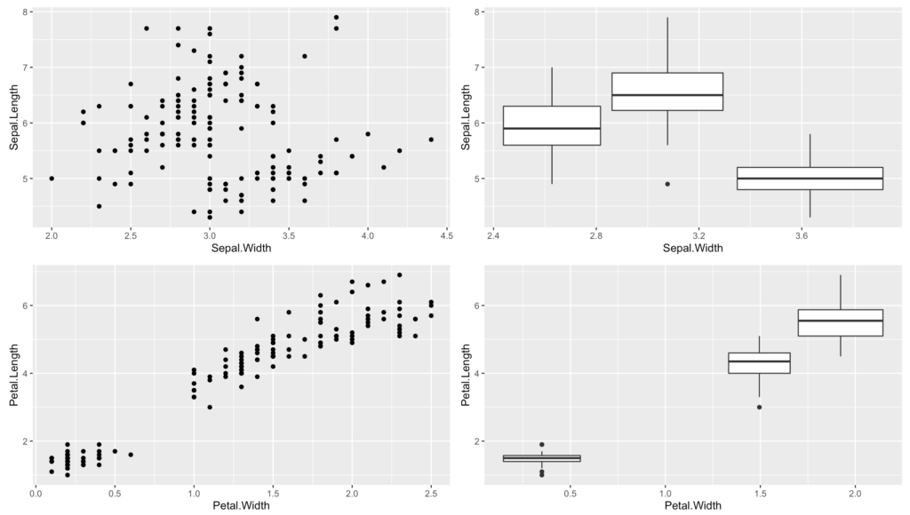
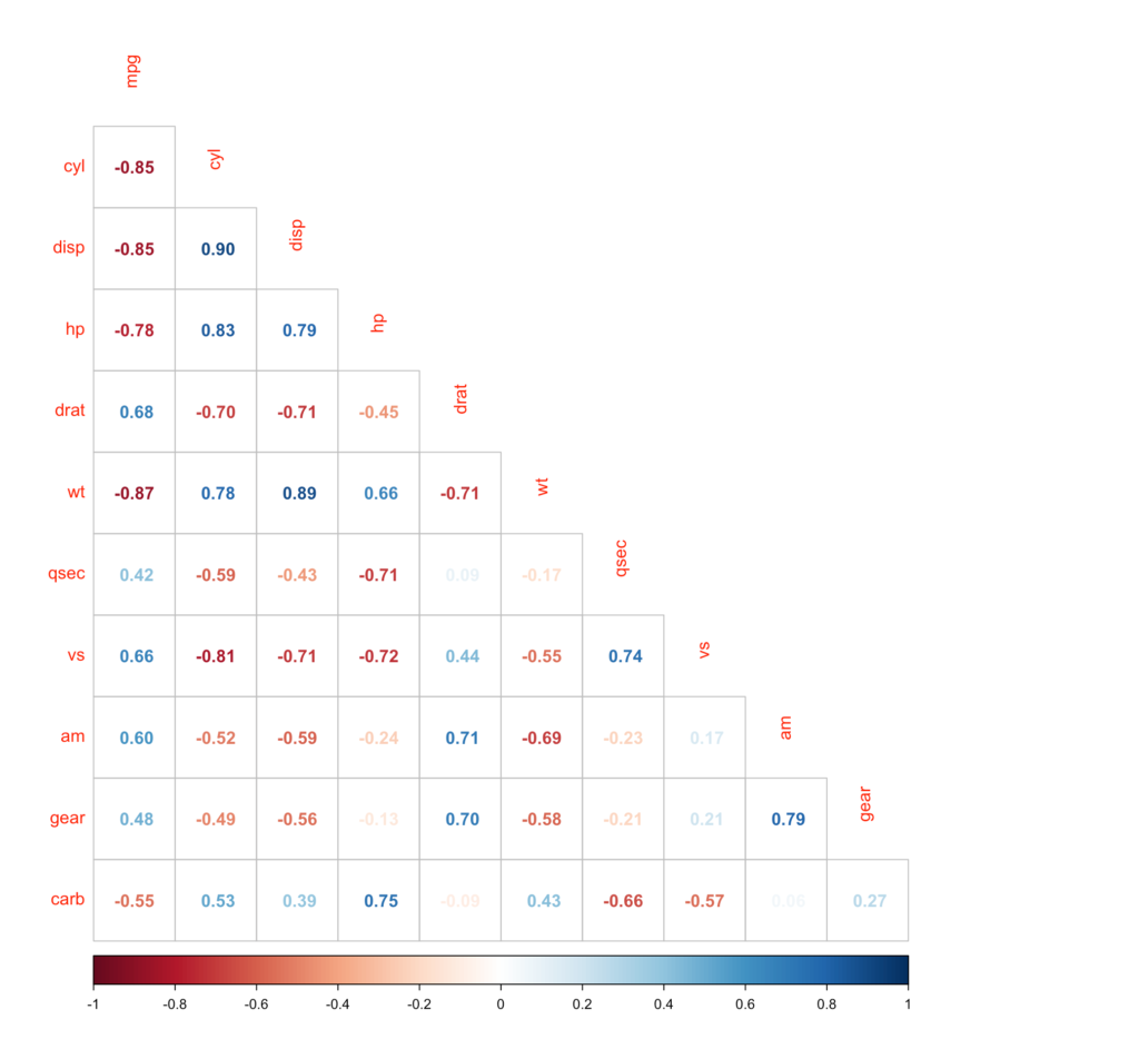
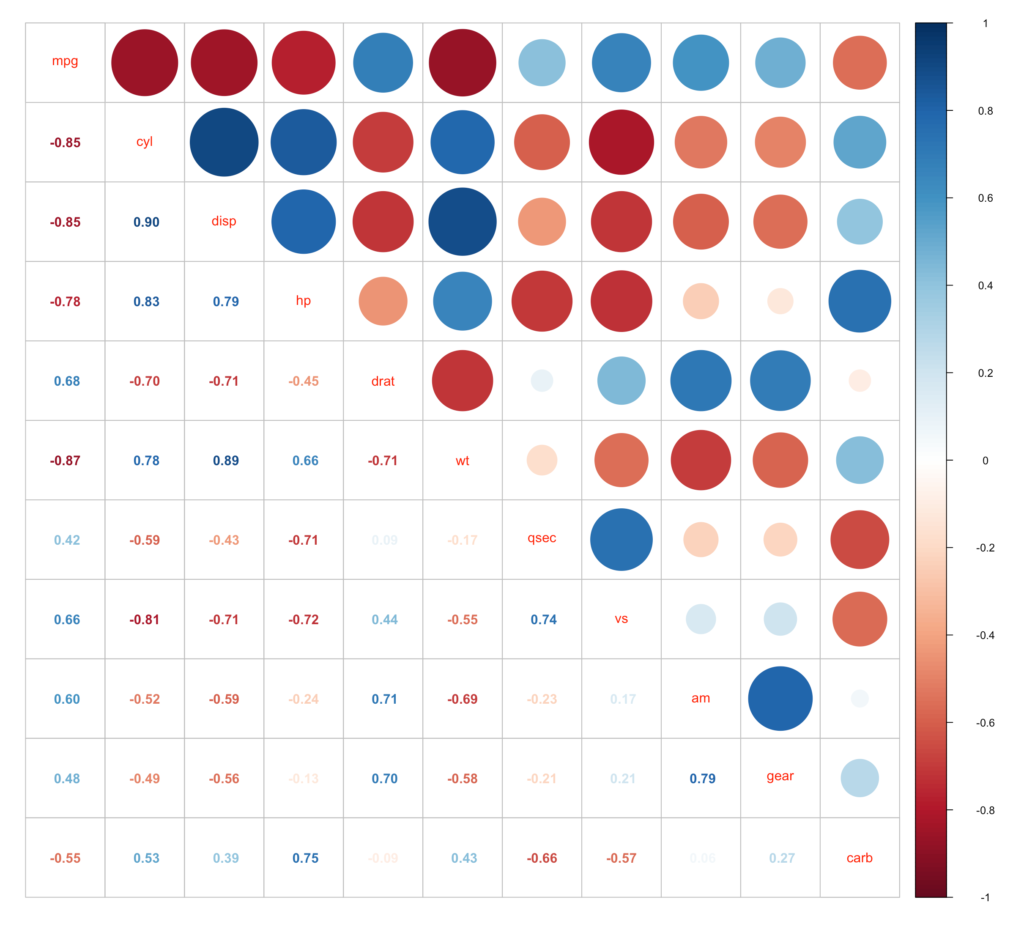
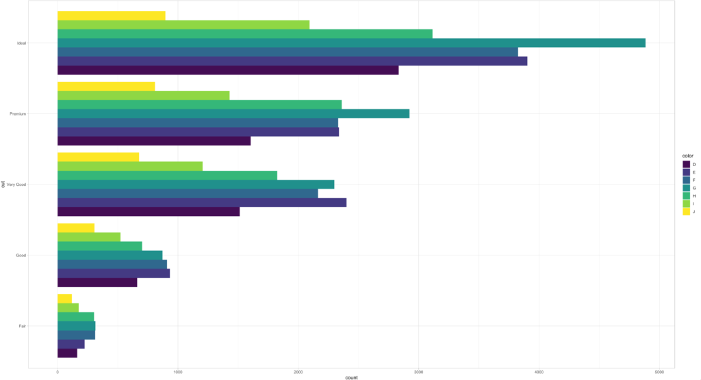
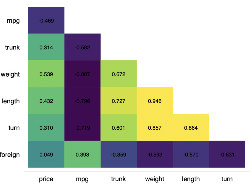
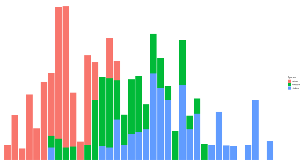
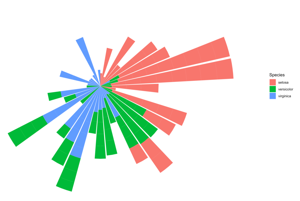
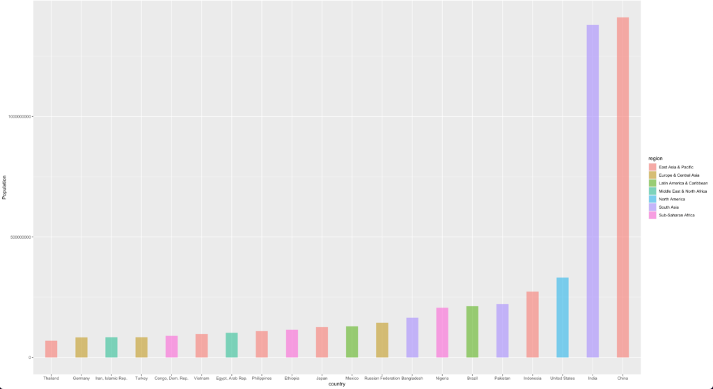
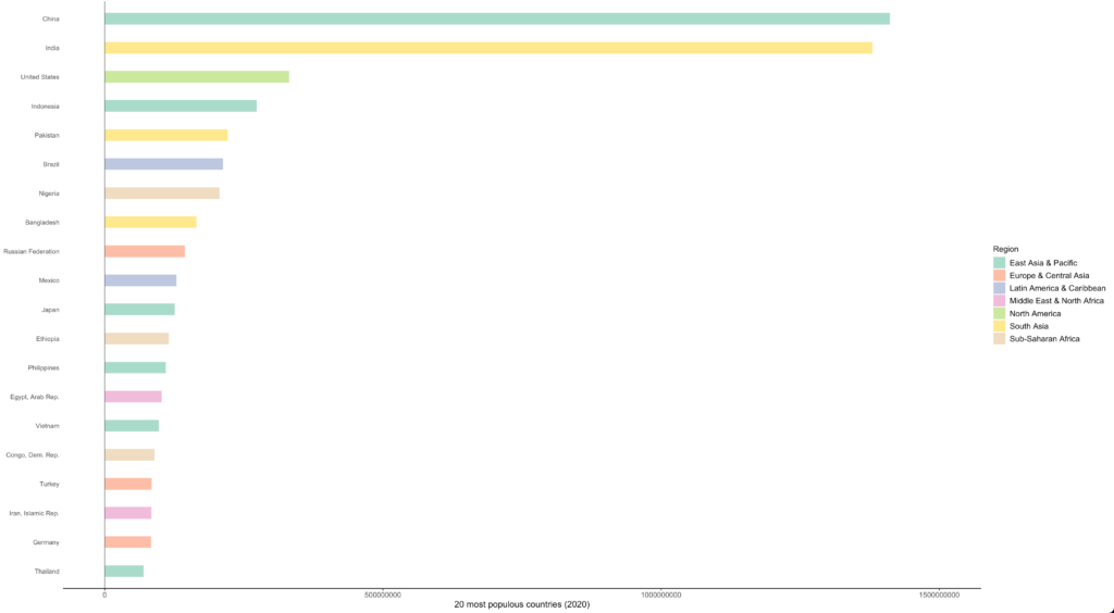
PDF files are embedded and may not display properly unless PDF viewer is enabled for the browser. Combining multiple plots in R #the librarylibrary(patchwork)#combine the plotsp1 <- ggplot(iris) + geom_point(aes(Sepal.Width, Sepal.Length))p2 <- ggplot(iris) + geom_boxplot(aes(Sepal.Width, Sepal.Length, group = Species))p3 <- ggplot(iris) + geom_point(aes(Petal.Width, Petal.Length))p4 <- ggplot(iris) + geom_boxplot(aes(Petal.Width, Petal.Length, group = Species))p1 + p2 + p3 + p4 Correlation plot in R #using the mtcars dataset#Plottinng coefs library(corrplot) cp = cor(mtcars) corrplot(cp, method = 'number', type = 'lower', diag = FALSE) #Plottinng both coefs and symbols corrplot.mixed(cp) Clustered bar chart in R #the librarylibrary(ggplot2)#making the plotggplot(data=diamonds) + geom_bar(mapping = aes(x=cut, fill = color), position="dodge")+ coord_flip()+ theme_light() Correlation plot in Stata #load a sample datasetsysuse auto, clear#create the correlation matrix:correlate price mpg trunk weight length turn foreignmatrix m = r(C)#plotheatplot C, values(format(%9.3f)) lower nodiagonal legend(off) sch(burd4) Changing to polar shape Coord polar chart in R #making the plot ggplot(data=diamonds) + geom_bar(mapping = aes(x=cut, fill = color), position="dodge")+ coord_flip()+ theme_light() Changing to polar shape p + coord_polar() Colouring indivudual bars in R Step 1: making the plot packages <- c( "tidyverse", "WDI", "forcats",'scales' ) pacman::p_load(packages, character.only = TRUE, install = FALSE) df <- WDI(indicator = "SP.POP.TOTL", start = 2020, end = 2020) country_code <- as_tibble(WDI_data$country) df <- df %>% rename(Population = SP.POP.TOTL) %>% inner_join(country_code, by = "iso2c") %>% filter(region != "Aggregates") %>% top_n(20, Population) %>% mutate(country = fct_reorder(country.x, Population)) p <- ggplot(df, aes(x = country, y = Population, fill = region)) + geom_bar(stat = "identity", alpha = .6, width = .4) p Step 2: Add additional features to the chart p+ coord_flip(ylim = c(10000, 1500000000)) + geom_hline(yintercept = 0, alpha = .5) + xlab("") + ylab("20 most populous countries (2020)") + theme_classic() + scale_fill_brewer(palette = "Set2", name = "Region") + theme( axis.line.y = element_blank(), axis.title.x = element_text(size = 12), axis.text.x = element_text(size = 10), axis.ticks.y = element_blank(), legend.text = element_text(size = 10) + scale_y_continuous(labels = function(x) format(x, scientific = FALSE)) ) Linear Regression Plot in R Logistic Regression Plot in R